2019 H2 Maths Paper 2, Question 10

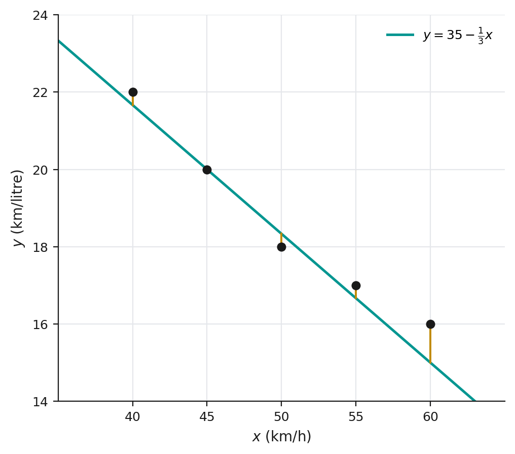
The five data points and Abi’s line $y = 35 - \frac{1}{3}x$ are plotted below.

For each point, the vertical segment down to (or up to) the line is the residual for that point, also shown on the diagram.

For each $x$, the value predicted by Abi’s line is $\widehat{y} = 35 - \frac{1}{3}x$, and each residual is $y - \widehat{y}$.

Sum of the squares of the residuals:

Explanation: Residuals above the line are positive and residuals below the line are negative, so in the sum of the residuals these can cancel out, giving a small (or even zero) total even when individual points lie far from the line. Squaring first removes the signs, so the sum of squares only shrinks when every point genuinely lies close to the line, making it a meaningful measure of the overall goodness of fit.

Since Bhani’s sum of squares of residuals, $1$, is less than Abi’s, $\frac{4}{3}$, Bhani’s line gives a better fit to the data.

$\therefore$ the least squares regression line must pass through $\left( \overline{x},\ \overline{y} \right)$.

Explanation: Here $\overline{x} = 50$ and $\overline{y} = 18.6$, so the line passes through $(50,\ 18.6)$.

By GC, the equation of the least squares regression line of $y$ on $x$ is

The product moment correlation coefficient is

Using the regression line, at $x = 30$,

$\therefore$ the estimated fuel consumption at a speed of $30\ km/h$ is $24.6\ km/\text{litre}$.

Explanation: This value is not expected to be reliable, since $x = 30$ lies outside the range of the given data ($40 \leq x \leq 60$), so the estimate requires extrapolation, and there is no evidence that the linear model still holds at that speed.

$\therefore$ all of Cerie’s data points lie exactly on her regression line, i.e. the points are perfectly collinear.

Explanation: A sum of squares of residuals of $0$ means every residual is $0$, so every data point lies exactly on the line.