 The Learning Cave
Part (a)
2 marksThere is a fairly strong negative linear correlation between distance driven, , and price, .
Explanation: the product moment correlation coefficient is negative and reasonably close to , so cars in this sample that have been driven further tend to have a lower price, and this decreasing relationship is reasonably well described by a straight line.
| To check your answer: on the scatter diagram, the point with the largest price () has the smallest distance (), and prices generally fall as distance increases across the rest of the points, consistent with a negative correlation. ✓ |
Part (b)
1 markThe PMCC would be unchanged; it would remain .
Explanation: converting units is a linear scaling of each variable — and , i.e. each variable is multiplied by a positive constant. The PMCC is unaffected by this kind of linear (origin-preserving, positive-scale) transformation of either variable.
Part (c)
1 markThis car should not be used in any analysis of the relationship between and for the standard model.
Explanation: being a special version with a bigger engine and extra features, it is not part of the same population as the rest of the data. Its price is likely to be higher for reasons unrelated to distance driven, so including it would bias any analysis of the relationship for the standard model.
Part (d)
5 marksWe exclude the special car and compute for the remaining cars.
We plot against and draw a line of best fit by eye.
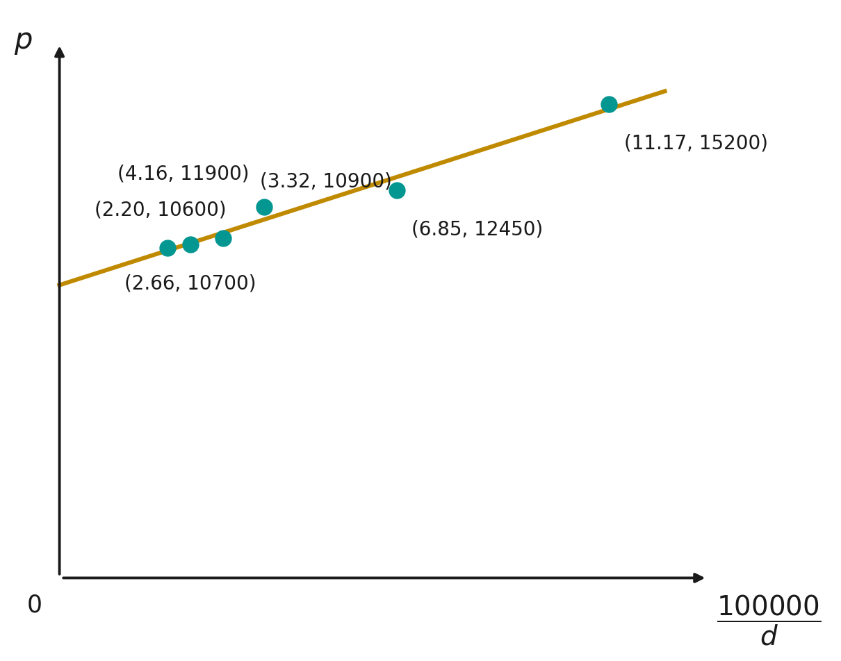
scatter diagram of against , with line of best fit as sketched above.
Part (e)
The distances used in the least squares regression line of on are the vertical distances from each plotted point to the line — that is, the difference between each observed price and the price predicted by the line at the corresponding .
These distances are squared so that points above and below the line (positive and negative deviations) do not cancel out when summed, and so that points further from the line are penalised more heavily than points close to it. The line is chosen to make the sum of these squared vertical distances as small as possible, which is why the procedure is called the method of least squares.
vertical distances from each point to the line are squared and summed; the line minimising this sum is the least squares regression line.
Part (f)
3 marksBy GC, performing linear regression of on for the remaining cars,
| To check your answer: with and , and , giving gradient and intercept , matching the GC output. ✓ |
(3 s.f. coefficients), (3 s.f.).
Part (g)
2 marksFor :
Substituting into the regression equation from (f):
This gives an estimated price of about £.
Explanation: this estimate is not likely to be reliable. The points used to fit the line have ranging only from about to , and lies well outside this range, so using the equation here is an extrapolation: the linear relationship may not hold beyond the data. Moreover, is exactly the special car excluded in (c), which is not of the standard specification the line was fitted to, so the estimate is doubly unreliable.
estimated price , but this is unreliable — it is an extrapolation, and the car is not of the standard specification.