2024 H2 Maths Paper 2 Q11 — Worked Solution

Part (a)(i)

1 mark

As $m$ increases, $p$ increases, but not at a constant rate: $p$ rises quickly for small $m$ and then more slowly as $m$ gets larger, so the rate of increase of $p$ decreases as $m$ increases.

Part (a)(ii)

6 marks

Approach

Both proposed models are linear in a transformed variable ( $\ln m$ or $\sqrt{m}$ ), so we find the product moment correlation coefficient for each transformed scatter plot and take the one closer to $\text{±}1$ as the better fit.

For the model $p = a + b\ln m$ , using the pairs $\left( \ln m,\ p \right)$ , by GC:

r = 0.9285\ \left( 4\ \text{d.p.} \right),\quad\quad a = - 703.8,\quad\quad b = 203.0

For the model $p = d + e\sqrt{m}$ , using the pairs $\left( \sqrt{m},\ p \right)$ , by GC:

r = 0.9914\ \left( 4\ \text{d.p.} \right),\quad\quad d = 32.95,\quad\quad e = 17.27

To check your answer: both correlation coefficients are close to

1

, consistent with the scatter diagram showing a strong relationship; the

\sqrt{m}

model’s is markedly closer to

1

, which matches the diagram levelling off much as

\sqrt{m}

does. ✓

Since $r$ for the $p = d + e\sqrt{m}$ model is closer to $1$ , this model gives the better fit.

$\therefore$ $p = 32.95 + 17.27\sqrt{m}$ , with $r = 0.9914$ .

Part (a)(iii)

Using $p = 32.95 + 17.27\sqrt{m}$ from (a)(ii) with $m = 750$ ,

p = 32.95 + 17.27\sqrt{750}

= 32.95 + 472.96

= 505.9

Correct to the nearest 10 cents, $p \approx 510$ cents.

Since $m = 750$ lies within the range of the given data ( $24 \leq m \leq 5000$ ), this estimate is an interpolation, so it is likely to be reliable.

$\therefore$ the estimated price is $510$ cents, and the estimate is reliable.

Part (b)(i)

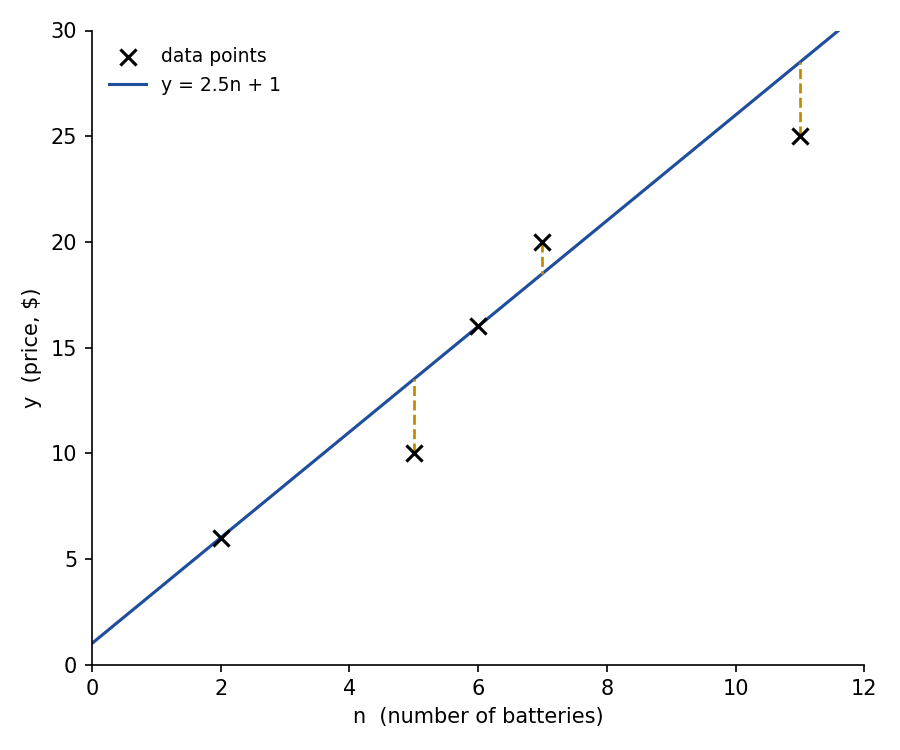
1 mark

The line $y = 2.5n + 1$ , together with the residual (dashed) for each data point, is:

Part (b)(ii)(A)

1 mark

The residual for each point is $y - f(n)$ , where $f(n) = 2.5n + 1$ :

$n$	2	5	6	7	11
$y$	6	10	16	20	25
$f(n)$	6	13.5	16	18.5	28.5
residual	0	$- 3.5$	0	1.5	$- 3.5$

These are the dashed vertical segments marked in the sketch in (b)(i).

Part (b)(ii)(B)

1 mark

Residuals can be positive or negative, so simply summing them could give a small (or even zero) total even when the model fits poorly, because positive and negative residuals cancel each other out. Squaring the residuals before summing removes this cancellation, so the sum reflects the true overall size of the deviations.

Part (b)(ii)(C)

2 marks

\text{Sum of squares} = 0^{2} + ( - 3.5)^{2} + 0^{2} + {1.5}^{2} + ( - 3.5)^{2}

= 0 + 12.25 + 0 + 2.25 + 12.25

= 26.75

To check your answer: the sum of the (unsquared) residuals is

0 - 3.5 + 0 + 1.5 - 3.5 = - 5.5 \neq 0

, as expected since

y = 2.5n + 1

was not obtained by least squares (a least-squares line always has residuals summing to

0

). ✓

$\therefore$ the sum of squares of residuals is $26.75$ .

Part (b)(iii)

A line that fits the data better has a smaller sum of squares of residuals than $26.75$ : the smaller the sum of squares, the better the fit.

Part (b)(iv)

3 marks

Approach

All lines $y = 2.5n + c$ share the same slope, so shifting $c$ shifts every residual by the same constant. Writing each residual for $y = 2.5n + c$ in terms of the $c = 1$ residuals lets us express the whole sum of squares as a single quadratic in $c$ , which we then compare against $26.75$ .

Let $d_{i} = y_{i} - 2.5n_{i}$ , the residual when $c = 0$ :

$n$	2	5	6	7	11
$d_{i} = y_{i} - 2.5n_{i}$	1	$- 2.5$	1	2.5	$- 2.5$

For general $c$ , the residual is $d_{i} - c$ , so the sum of squares is

S(c) = \sum\left( d_{i} - c \right)^{2}

= \sum d_{i}^{2} - 2c\sum d_{i} + 5c^{2}

\sum d_{i} = 1 - 2.5 + 1 + 2.5 - 2.5 = - 0.5,\quad\quad\sum d_{i}^{2} = 1 + 6.25 + 1 + 6.25 + 6.25 = 20.75

S(c) = 20.75 + c + 5c^{2}

To check your answer:

S(1) = 20.75 + 1 + 5 = 26.75

, matching (b)(ii)(C) exactly, since

c = 1

gives back the original line

y = 2.5n + 1

. ✓

We require $S(c) < S(1) = 26.75$ :

20.75 + c + 5c^{2} < 26.75

\Rightarrow 5c^{2} + c - 6 < 0

c = \frac{- 1 \pm \sqrt{1 + 120}}{10}

= \frac{- 1 \pm 11}{10}

= 1\ \text{or}\ - 1.2

Since the graph of $5c^{2} + c - 6$ against $c$ is an upward parabola, it is negative between its roots.

$\therefore$ $- 1.2 < c < 1$ .

2024 H2 Maths Paper 2, Question 11

Part (a)(i)

Part (a)(ii)

Part (a)(iii)

Part (b)(i)

Part (b)(ii)(A)

Part (b)(ii)(B)

Part (b)(ii)(C)

Part (b)(iii)

Part (b)(iv)

This is how we mark, and how we teach.